Excel : How To Remove First, Last Or Certain Characters From Text In Excel?

Remove First Or Last Characters By Formula In Excel

With the Excel LEFT and RIGHT function, you can remove the certain characters from the beginning or the end of the strings. Please do as the following steps:

Remove the first four characters from the text string.

Step 1. Type the following formula in adjacent cell B1: =RIGHT(A1, LEN(A1)-4), see screenshot:



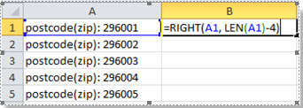
Tips: This formula means to return the right most number of characters, you need to subtract 4 characters from left string. And you can specify the number of characters you want to remove from the left string by changing the Number 4 in the formula =RIGHT(A1, LEN(A1)-4).

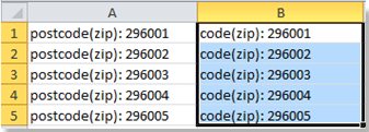
Step 2. Then press Enter key, and select the cell B1, then drag the fill handle over the cells that you want to contain this formula. And now you are successful in removing the first 4 characters of the text strings. See screenshot:



If you need to remove the last several characters, you can use the LEFT function as the same as the RIGHT function.

Note: Using the Excel function to remove certain characters is not as directly as it is. Just take a look at the way provided in next method, which is no more than two or three mouse clicks.

Remove First Or Last Characters By Find And Replace In Excel

If you want to remove all characters at the front or end of the colon :, Find and Replace function in Excel also can make your removing as soon as quickly.

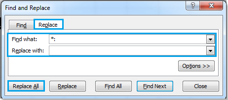
Step 1. Hold the Ctrl button and press F to open Find and Replace dialog, and click Replace.

Step 2. Enter :* into the Find what box, and leave blank in Replace with box. See screenshot:



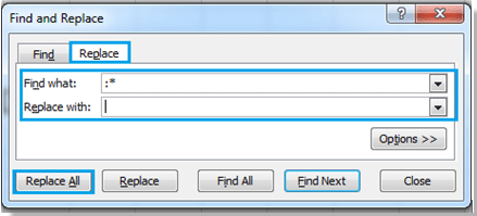
Step 3. Click Replace All, and all the characters at the end of the colon (include the colon) have been removed. See screenshot:



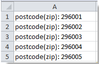
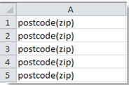
If you want to remove all characters before the colon, please type *: into the Find what box, and leave blank in Replace with box. See screenshot:



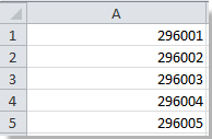
Click Replace All, all the characters before the colon have been removed. See screenshot:



Note: This method is only applied to the characters which contain the specific separators, so you can change the colon: to any other separators as your need.

https://www.extendoffice.com/documents/excel.html

Excel : How To Move Minus Sign From Right To Left/Back To Front In Excel?

Symptoms

When you import a worksheet into Microsoft Excel and that worksheet contains numbers with minus signs on the right (for example, 12345-), Microsoft Excel may not treat these numbers as negative numbers.

Cause

Microsoft Excel treats these numbers as text because the minus sign appears to the right side of the number.

Workaround

There are two ways to solve this problem:

1. Use a worksheet formula. -or-

2. Create a macro.

Use the following formula in a worksheet:

=IF(RIGHT(A1,1)="-","-"&LEFT(A1,LEN(A1)-1),A1)*1
=IF(RIGHT(A1,1)="-",SUBSTITUTE(A1,"-","")*-1,A1)
=VALUE(IF(RIGHT(A1,1)="-",RIGHT(A1,1)&LEFT(A1,LEN(A1)-1),A1))

For example, follow these steps:

1. Enter the following in a worksheet:

A1: 3

A2: 2-

A3: 1-

A4: 4

A5: 6-

2. In cell B1, enter the above formula.

3. Fill the formula in B1 down to B5.

4. Select cells B1:B5 and click Copy on the Edit menu.

5. Select cell A1 and click Paste Special on the Edit menu.

6. Click Values and click OK.

7. Select B1:B5 and click Delete on the Edit menu.

*******************************************************************************

There is a hidden utility in Text to Columns that can help you move minus sign from back to front.

1. Select the numbers you want to fix the trailing minus sign, and click Data à Text to Columns. 

2. In the Text to Columns wizard, directly click Next à Next to go to the Step 3 of 3 dialog, and click Advanced. 

3. In the Advanced Text Import Settings dialog, just check Trailing minus for negative numbers option, and click OK to close it.

4. Then click Finish to close Text to Columns dialog, and the minus sign of the negative numbers have been moved from back to front.

*******************************************************************************

If you are familiar with VBA, here is one can help you.

1. Press Alt + F11 keys simultaneously to open Microsoft Visual Basic for Applications window.

2. Click Insert à Module, and paste below VBA code to the new Module window.

VBA: Move minus sign from back to front (right to left)

Sub FixTrailingNumbers()

'UpdatebyKutoolsforExcel20160409

    Dim xRg As Range

    Dim xCol As Range

    Dim xTxt As String

    On Error Resume Next

    xTxt = ActiveWindow.RangeSelection.Address

    Set xRg = Application.InputBox("Select a range", "Kutools for Excel", xTxt, , , , , 8)

    If xRg Is Nothing Then Exit Sub

    For Each xCol In xRg.Columns

        xCol.TextToColumns Destination:=xCol, TrailingMinusNumbers:=True

    Next

End Sub

3. Click Run button or F5 key to execute this code, and a Kutools for Excel dialog pops out to remind you select a range to work. 

4. Click OK, and now the minus signs of negative numbers have been fixed correctly.

------------------***************------------------

https://www.extendoffice.com/documents/excel.html

Outlook: “Can’t Create File” Error When Opening Attachment

When you try to open a file attachment in Microsoft Outlook, you get an error:

Cause : 
This issue may occur when the Temporary Internet Files folder is stored on a server on which you do not have sufficient permissions.

Symptoms :
When you try to open or save an e-mail attachment, you may receive the following error message:
Cannot create file: file name. Right-click the folder you want to create the file in and click Properties on the shortcut menu to check your permissions for the folder.

Steps:

This problem occurs usually when Outlook cannot access the temp file the file is linked to. To resolve this problem, try the following steps.

1. Hold the Windows Key, then press “R” to bring up the Run dialog box.

2. Type “Regedit“, then press “Enter“.

3. Click “Edit” > “Find” and type “OutlookSecureTempFolder“.

4. When regedit has found the entry, it will tell you where your Outlook temporary files are stored. It will look similar to one of the following:

C:\Users\username\AppData\Local\Microsoft\Windows\INetCache\ Content.Outlook\randomnumber\

C:\Documents and Settings\username\Local Settings\Temporary Internet Files\OLKrandomnumber

5. Bring up the File Explorer, then navigate to the location in the registry key.

6. Delete all of the files in this folder.

7. Restart Microsoft Outlook and you should be able to open your attachment.

Excel : Shortcut Keys

Home --> Font : Alt + H 

Figure 1: Borders --> Alt + H + B

Figure 2: Theme & Standard colors --> Alt + H + H

Figure 3: Automatic --> Theme & Standard colors --> Alt + H + FC

Figure 4: Format Cells --> Alt + H + FN   (or)   Ctrl + Shift + F

Figure 5: Bold --> Alt + H + 1 (or) Ctrl + B

Excel : Text to Columns

To separate the contents of one Excel cell into separate columns, you can use the 'Convert Text to Columns Wizard'.

1. Select the range with full Column A.

2. On the Data tab, click Text to Columns.

The following dialog box appears.

3. Choose Delimited and click Next.



4. Clear all the check boxes under Delimiters except for the Other check box.

5. Click Next 

6. Select Column data format.

7. Click Next.

Note: This example has commas and spaces as delimiters. You may have other delimiters in your data. Experiment by checking and unchecking the different check boxes. You get a live preview of how your data will be separated.

Result:

Protect Macro

Command Button:-

Place a "Command Button" on your worksheet and add the following code lines:

1. On the Developer tab, click Insert.

2. In the ActiveX Controls group, click Command Button.



3. Drag a command button on your worksheet.

Assign a Macro:-

To assign a macro (one or more code lines) to the command button, execute the following steps.

1. Right click CommandButton1 (make sure Design Mode is selected).

2. Click View Code.



The Visual Basic Editor appears.

3. Place your cursor between Private Sub CommandButton1_Click() and End Sub.

4. Add the code line shown below.


Protect Macro

1. First, create a simple macro that you want to protect.

Range("A1").Value = "This is secret code"

2. Next, click Tools, VBAProject Properties...



3. On the Protection tab, check "Lock project for viewing" and enter a password twice.



4. Click OK.

5. Save, close and reopen the Excel file. Try to view the code.

The following dialog box will appear:



You can still execute the code by clicking on the command button but you cannot view or edit the code anymore (unless you know the password). The password for the downloadable Excel file is "easy".

6. If you want to password protect the macro from being executed, add the following code lines:

Dim password As Variant
password = Application.InputBox("Enter Password", "Password Protected")

Select Case password
    Case Is = False
        'do nothing
    Case Is = "easy"
        Range("A1").Value = "This is secret code"
    Case Else
        MsgBox "Incorrect Password"
End Select



Result when you click the command button on the sheet:

How to protect Excel sheet

To protect a sheet in Excel 2016, 2013 and 2010, perform the following steps.

1. Right click a worksheet tab at the bottom of your screen and select Protect Sheet… from the context menu.

Or, click the Protect Sheet button on the Review tab, in the Changes group.



2. In the Protect Sheet dialog window, do the following:

To password protect your Excel sheet, type a password in the corresponding field. Be sure to remember the password or store it in a safe location because you will need it later to unprotect the sheet.

If the worksheet protection is nothing more than a precaution against accidental modification of the sheet contents by yourself or by the members of your local team, you may not want to bother about memorizing the password and leave the password field empty. In this case, unprotecting the sheet takes just a single click on the Unprotect Sheet button on the ribbon or in the sheet tab's right-click menu.

Select the actions you allow the users to perform.

• By default, the following 2 options are selected: Select locked cells and Select unlocked cells. If you leave only these two options selected, the users of your sheet, including yourself, will be able only to select cells (both locked and unlocked).
• To allow some other actions such as sorting, filtering, formatting cells, deleting or inserting rows and columns, check the corresponding boxes.
• If you don't check any action, users will only be able to view the contents of your Excel sheet.

Click the OK button.



3. The Confirm Password dialog box will pop-up prompting you to retype the password so that an accidental misprint won't lock your Excel sheet forever. Retype the password and click OK. Done!

How to unprotect Excel sheet with password

If you know the password for the protected sheet, removing protection is a matter of seconds. Just do any of the following:

1. Right-click the sheet tab, and select Unprotect Sheet… from the context menu.



2. On the Review tab, in the Changes group, click Unprotect Sheet.



3. On the Home tab, in the Cells group, click Format, and select Unprotect Sheet from the drop-down menu.



If you are dealing with a password-protected worksheet, Excel will ask you to enter the password. Type the password and click OK.

If the worksheet was not protected with password, clicking the Unprotect Sheet button is all it takes to unlock the sheet.

How to unprotect Excel sheet without password

As mentioned in the beginning of this tutorial, Excel worksheet protection is quite weak even in the recent versions of Excel 2013 and Excel 2016. If you need to edit a password protected sheet but you cannot remember the password, try to unlock that Excel spreadsheet by using one of the following methods.

Unlock Excel spreadsheet with VBA code (for Excel 2010 and lower) :-

If you are using Excel 2010 or older version, you can unlock a password-protected sheet with the following macro.

1. Press Alt + F11 to open the Visual Basic Editor.



2. Right-click the workbook name on the left pane (Project-VBAProject pane) and select Insert > Module from the context menu.



3. Copy and paste the code below into the (Code) window. Do not change any of the code, just copy and paste it.

Sub PasswordBreaker()
    'Breaks worksheet password protection.
    Dim i As Integer, j As Integer, k As Integer
    Dim l As Integer, m As Integer, n As Integer
    Dim i1 As Integer, i2 As Integer, i3 As Integer
    Dim i4 As Integer, i5 As Integer, i6 As Integer
    On Error Resume Next
    For i = 65 To 66: For j = 65 To 66: For k = 65 To 66
    For l = 65 To 66: For m = 65 To 66: For i1 = 65 To 66
    For i2 = 65 To 66: For i3 = 65 To 66: For i4 = 65 To 66
    For i5 = 65 To 66: For i6 = 65 To 66: For n = 32 To 126
        ActiveSheet.Unprotect Chr(i) & Chr(j) & Chr(k) & _
            Chr(l) & Chr(m) & Chr(i1) & Chr(i2) & Chr(i3) & _
            Chr(i4) & Chr(i5) & Chr(i6) & Chr(n)
        If ActiveSheet.ProtectContents = False Then
            MsgBox "One usable password is " & Chr(i) & Chr(j) & _
                Chr(k) & Chr(l) & Chr(m) & Chr(i1) & Chr(i2) & _
                Chr(i3) & Chr(i4) & Chr(i5) & Chr(i6) & Chr(n)
            Exit Sub
        End If
    Next: Next: Next: Next: Next: Next
    Next: Next: Next: Next: Next: Next
End Sub

4. Press F5 or click the Run button on the toolbar and wait a couple of minutes. The macro will report a cracked password, which is not the original one (always some combination of A's and B's), but nevertheless it works. If you are not very comfortable with VBA, you can find the detailed guidance in the following tutorial: How to insert and run VBA code in Excel. If you need to unprotect Excel sheet without password in the modern versions of Excel 2013 and Excel 2016, try one of free tools, for example Password Protection Remover add-in for Excel.

4. Save your workbook as "Excel macro-enabled workbook". Press Crl+S, then click the "No" button in the "The following features cannot be saved in macro-free workbook" warning dialog.

The "Save as" dialog will open. Choose "Excel macro-enabled workbook" from the "Save as type" drop-down list and click the Save button.

5. Press Alt+Q to close the Editor window and switch back to your workbook.

How to run VBA macros in Excel

When you want to run the VBA code that you added as described in the section above: press Alt+F8 to open the "Macro" dialog.

Then select the wanted macro from the "Macro Name" list and click the "Run" button.

https://www.ablebits.com/office-addins-blog/2013/12/06/add-run-vba-macro-excel/