How To Spell Out Or Convert Numbers To English Words In Excel?

Supposing you have a lot of price amount numbers, and now you need to convert or spell out them to text strings. For example, convert 123.55 to the English words one hundred twenty-three dollars and fifty five cents. In Excel there are no effective facility to solve this problem but using the long and complex VBA code. In this article, I will introduce you some methods to deal with it.

Spell Out Or Convert Numbers To English Words With VBA Code

The following long VBA code can help you to spell out numbers to text strings. Do as follows:

1. Hold down the ALT + F11 keys, and it opens the Microsoft Visual Basic for Applications window.

2. Click Insert > Module, and paste the following macro in the Modulewindow.

Function SpellNumberToEnglish(ByVal pNumber)
'Updateby20131113
Dim Rupees, paise
arr = Array("", "", " Thousand ", " Million ", " Billion ", " Trillion ")
pNumber = Trim(Str(pNumber))
xDecimal = InStr(pNumber, ".")
If xDecimal > 0 Then
    paise = GetTens(Left(Mid(pNumber, xDecimal + 1) & "00", 2))
    pNumber = Trim(Left(pNumber, xDecimal - 1))
End If
xIndex = 1
Do While pNumber <> ""
    xHundred = ""
    xValue = Right(pNumber, 3)
    If Val(xValue) <> 0 Then
        xValue = Right("000" & xValue, 3)
        If Mid(xValue, 1, 1) <> "0" Then
            xHundred = GetDigit(Mid(xValue, 1, 1)) & " Hundred "
        End If
        If Mid(xValue, 2, 1) <> "0" Then
            xHundred = xHundred & GetTens(Mid(xValue, 2))
        Else
            xHundred = xHundred & GetDigit(Mid(xValue, 3))
        End If
    End If
    If xHundred <> "" Then
        Rupees = xHundred & arr(xIndex) & Rupees
    End If
    If Len(pNumber) > 3 Then
        pNumber = Left(pNumber, Len(pNumber) - 3)
    Else
        pNumber = ""
    End If
    xIndex = xIndex + 1
Loop
Select Case Rupees
    Case ""
        Rupees = "No Rupees"
    Case "One"
        Rupees = "One Dollar"
    Case Else
        Rupees = Rupees & " Rupees"
End Select
Select Case paise
    Case ""
        paise = " and No paise"
    Case "One"
        paise = " and One paise"
    Case Else
        paise = " and " & paise & " paise"
End Select
SpellNumberToEnglish = Rupees & paise
End Function
Function GetTens(pTens)
Dim Result As String
Result = ""
If Val(Left(pTens, 1)) = 1 Then
    Select Case Val(pTens)
        Case 10: Result = "Ten"
        Case 11: Result = "Eleven"
        Case 12: Result = "Twelve"
        Case 13: Result = "Thirteen"
        Case 14: Result = "Fourteen"
        Case 15: Result = "Fifteen"
        Case 16: Result = "Sixteen"
        Case 17: Result = "Seventeen"
        Case 18: Result = "Eighteen"
        Case 19: Result = "Nineteen"
        Case Else
    End Select
Else
Select Case Val(Left(pTens, 1))
    Case 2: Result = "Twenty "
    Case 3: Result = "Thirty "
    Case 4: Result = "Forty "
    Case 5: Result = "Fifty "
    Case 6: Result = "Sixty "
    Case 7: Result = "Seventy "
    Case 8: Result = "Eighty "
    Case 9: Result = "Ninety "
    Case Else
End Select
Result = Result & GetDigit(Right(pTens, 1))
End If
GetTens = Result
End Function
Function GetDigit(pDigit)
Select Case Val(pDigit)
    Case 1: GetDigit = "One"
    Case 2: GetDigit = "Two"
    Case 3: GetDigit = "Three"
    Case 4: GetDigit = "Four"
    Case 5: GetDigit = "Five"
    Case 6: GetDigit = "Six"
    Case 7: GetDigit = "Seven"
    Case 8: GetDigit = "Eight"
    Case 9: GetDigit = "Nine"
    Case Else: GetDigit = ""
End Select
End Function

3. Then save the code, and return to the worksheet, in the adjacent cell C2, enter the formula =SpellNumberToEnglish(A2), see screenshot:

4. Then press Enter key, and select the cell C2, then drag the fill handle over to the range that contains this formula as you need. And all of the numbers have been spelt out to English words. See screenshot:

Note: As they are formulas, when you need to copy and paste them, please paste as values.

Link: https://www.extendoffice.com/documents/excel/1142-excel-spell-out-numbers.html

How To Quickly Convert / Change Numbers To Words In Excel?

If you have a column of numeric values in a worksheet, and now you need to convent them to their equivalent English words (as following screenshot shown). Here I will talk about a method to change the numbers to English words quickly and easily.

Convert Numbers To English Words With User Defined Function

There are no features or formulas can help you to solve this task directly in Excel, but you can create a User Defined Function to finish it. Please do with following steps:

1. Hold down the ALT + F11 keys, and it opens the Microsoft Visual Basic for Applications Window.

2. Click Insert > Module, and paste the following code in the Module Window.

Function NumberstoWords(ByVal pNumber)

'Updateby20140220

Dim Rupees

arr = Array("", "", " Thousand ", " Million ", " Billion ", " Trillion ")

pNumber = Trim(Str(pNumber))

xDecimal = InStr(pNumber, ".")

If xDecimal > 0 Then

pNumber = Trim(Left(pNumber, xDecimal - 1))

End If

xIndex = 1

Do While pNumber <> ""

xHundred = ""

xValue = Right(pNumber, 3)

If Val(xValue) <> 0 Then

xValue = Right("000" & xValue, 3)

If Mid(xValue, 1, 1) <> "0" Then

xHundred = GetDigit(Mid(xValue, 1, 1)) & " Hundred "

End If

If Mid(xValue, 2, 1) <> "0" Then

xHundred = xHundred & GetTens(Mid(xValue, 2))

Else

xHundred = xHundred & GetDigit(Mid(xValue, 3))

End If

End If

If xHundred <> "" Then

Rupees = xHundred & arr(xIndex) & Rupees

End If

If Len(pNumber) > 3 Then

pNumber = Left(pNumber, Len(pNumber) - 3)

Else

pNumber = ""

End If

xIndex = xIndex + 1

Loop

NumberstoWords = Rupees

End Function

Function GetTens(pTens)

Dim Result As String

Result = ""

If Val(Left(pTens, 1)) = 1 Then

Select Case Val(pTens)

Case 10: Result = "Ten"

Case 11: Result = "Eleven"

Case 12: Result = "Twelve"

Case 13: Result = "Thirteen"

Case 14: Result = "Fourteen"

Case 15: Result = "Fifteen"

Case 16: Result = "Sixteen"

Case 17: Result = "Seventeen"

Case 18: Result = "Eighteen"

Case 19: Result = "Nineteen"

Case Else

End Select

Else

Select Case Val(Left(pTens, 1))

Case 2: Result = "Twenty "

Case 3: Result = "Thirty "

Case 4: Result = "Forty "

Case 5: Result = "Fifty "

Case 6: Result = "Sixty "

Case 7: Result = "Seventy "

Case 8: Result = "Eighty "

Case 9: Result = "Ninety "

Case Else

End Select

Result = Result & GetDigit(Right(pTens, 1))

End If

GetTens = Result

End Function

Function GetDigit(pDigit)

Select Case Val(pDigit)

Case 1: GetDigit = "One"

Case 2: GetDigit = "Two"

Case 3: GetDigit = "Three"

Case 4: GetDigit = "Four"

Case 5: GetDigit = "Five"

Case 6: GetDigit = "Six"

Case 7: GetDigit = "Seven"

Case 8: GetDigit = "Eight"

Case 9: GetDigit = "Nine"

Case Else: GetDigit = ""

End Select

End Function

3. Save and close this code and go back the worksheet, in a blank cell, enter this formula =NumberstoWords(A2)( A2 is the cell you want to convert the number to English word), see screenshot:

4. Then press Enter key, and select cell C2 then drag the fill handle to the range that you want to contain this formula. All the numeric values have been converted their corresponding English words.

Note: When you need to copy these results to other cells, please copy and paste them as Values.

Link: https://www.extendoffice.com/documents/excel/1446-excel-convert-change-numbers-to-words.html

Excel : Freezing Panes

To freeze rows:

You may want to see certain rows or columns all the time in your worksheet, especially header cells. By freezing rows or columns in place, you'll be able to scroll through your content while continuing to view the frozen cells.

1. Click the View tab on the Ribbon.

2. Select the Freeze Panes command, then choose Freeze Panes from the drop-down menu.

3. Select the row below the row(s) you want to freeze. In our example, we want to freeze rows 1, so we'll select row 2.

To freeze columns:

4. Select the column to the right of the column(s) you want to freeze. In our example, we want to freeze column A, so we'll select column B.

To freeze columns & rows:

5. If you only need to freeze the top row (row 1) or first column (column A) in the worksheet, you can simply select Freeze Top Row or Freeze First Column from the drop-down menu.

Note: To unfreeze rows or columns, click the Freeze Panes command, then select Unfreeze Panes from the drop-down menu.

Excel : Split Worksheet Into Panes With Split Button

1. Select the row you want to insert the split pane above it firstly.

Tip: If you want to insert vertical split pane, you can select a column you want to insert the split pane left to it.

2. Then click View > Split, and you can see the split pane is inserted into the worksheet.

Tip: If you want to insert a cross split pane into a worksheet, select a cell that you want to insert horizontal split pane above and the vertical split pane left to, then click View > Split. 

Note: If you want to clear the split panes, just double click the pane you want to delete, then it will be removed.

Excel : Stop Excel from Checking for Errors in the Background

While you have Excel open, it is constantly checking in the background for potential errors in your worksheets. If an error is located (or, at the least, what Excel thinks is an error), then the cell is "flagged" with a small green triangle in the upper-left corner of the cell.

If you don't want Excel to check for errors, you can turn the feature off by following these steps:

1. Click the File tab at the top-left corner of the window.

2. Display the Excel Options dialog box. (In Excel 2007 click the Office button and then click Excel Options. In Excel 2010 and Excel 2013 display the File tab of the ribbon and then click Options.)

3. Click Formulas at the left side of the dialog box. (See Figure 1.)

Figure 1. The Formulas area of the Excel Options dialog box.

4. Click the box to the left of Enable background error checking to remove the check mark. You can then click the OK button at the bottom of the window to apply your changes.

5. Result..

How to Recover Bit Locker Encrypted Disks Should You Forget Your Password

Option One:- 

To Unlock a Data or Removable Drive Using BitLocker Wizard

1. Open the Control Panel -> System and security, click on the BitLocker Drive Encryption icon, and click on the Unlock Drive link for the locked drive that you would like to unlock. (see screenshot below)

2. Click on Unlock Drive.... (see screenshot below)

3. Click on the I forgot my password link. (see screenshot below)

4. Using the provided "recovery key ID" number in the screenshot below, locate the BitLocker recovery key for this drive, and then click on Type the recovery key. (see screenshots below)

5. Type in the long BitLocker recovery key number, and click on Next. (see screenshot below)

6. Click on Finish, and continue on to step 7. (see screenshot below)

NOTE: If you had forgotten the password, then you can now click on Manage BitLocker, and Change password to unlock drive to create a new one to use.

7. The drive will now be unlocked until you log off or restart the computer next.

Option Two:-

To Unlock a Data or Removable Drive in a Command Prompt

1. Open a elevated command prompt.

2. To Use the "BitLocker Recovery Key" to Unlock this Drive

NOTE: This step is for if you lost or forgot the password for this drive.

A) Locate the BitLocker recovery key for this drive. (see screenshots below)

NOTE: Substitute E: in the command below with the drive letter of the locked drive that you wanted to unlock, and substitute BitLocker Recovery Key in the command below with the actual long number recovery key for the drive.

manage-bde -unlock D: -rp BitLocker Recovery Key

BitLocker Drive Encryption - Unlock a Locked Data or Removable Drive-cmd-recovery_key.jpg

C) Go to step 4.

4. The drive will now be unlocked until you log off or restart the computer next. 

How to Lock Folder Through Command

Step 1.
1. Press Win+R in your keyboard (To bring Run command tool)
2. Then type: Notepad
3. Press enter.

Step 2.
You will see notepad
Now type the Codes/Command.

Step 3.
SO THE CODES ARE HERE:
cls
@ECHO OFF
title Folder Locker
if EXIST "Control Panel.{21EC2020-3AEA-1069-A2DD-08002B30309D}" goto UNLOCK
if NOT EXIST secured goto MDLOCKER
:CONFIRM
echo Are you sure u want to Lock the secured(Y/N)
set/p "cho=>"
if %cho%==Y goto LOCK
if %cho%==y goto LOCK
if %cho%==n goto END
if %cho%==N goto END
echo Invalid choice.
goto CONFIRM
:LOCK
ren secured "Control Panel.{21EC2020-3AEA-1069-A2DD-08002B30309D}"
attrib +h +s +r +i "Control Panel.{21EC2020-3AEA-1069-A2DD-08002B30309D}"
echo secured locked
goto End
:UNLOCK
echo put in the key to Unlock the lock
set/p "pass=>password"
if NOT %pass%==123456 goto FAIL
attrib -h -s "Control Panel.{21EC2020-3AEA-1069-A2DD-08002B30309D}"
ren "Control Panel.{21EC2020-3AEA-1069-A2DD-08002B30309D}" secured
echo secured Unlocked
goto End
:FAIL
echo Invalid keyword
goto UNLOCK
:MDLOCKER
md Secured
echo lock unlocked
goto End
:End

NOTE: In 23rd Line You can see the default password i.e., 123456 , so just change this to the password you want.

- So Just write The Codes In a same Way it is written And Save as "all file" type with file name lock.bat or anything.bat

Step 4:
1. When you open that Lock.bat file, it will create one folder name Secured 
2. So, copy any files or folders you want to hide and paste/move it to secured folder.

Step 5:
1. Now, again open that bat file and you will see that
2. Asking to lock or not. so, if you want to lock type:Y
3. And the press enter, now you folder is locked or hidden.

Bug: Some Of The Users Told Me That during This Step 5 when we lock the folder, the folder is still seen...

Bug Fixed: So Just Refresh (Press Ctrl+F5) it once in desktop or in the location where you are trying to lock that file...

Step 6:
1. In order to get your file back, open the bat file again. So now you can see something like this
2. Since here the default password i set is 123456, which you can change easily before running the program, which i already explained in Step 3.
3. Press enter, you file will be right there.

http://www.instructables.com/id/How-To-Lock-Folder-Through-CMD/

Excel : How To Remove First, Last Or Certain Characters From Text In Excel?

Remove First Or Last Characters By Formula In Excel

With the Excel LEFT and RIGHT function, you can remove the certain characters from the beginning or the end of the strings. Please do as the following steps:

Remove the first four characters from the text string.

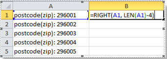
Step 1. Type the following formula in adjacent cell B1: =RIGHT(A1, LEN(A1)-4), see screenshot:



Tips: This formula means to return the right most number of characters, you need to subtract 4 characters from left string. And you can specify the number of characters you want to remove from the left string by changing the Number 4 in the formula =RIGHT(A1, LEN(A1)-4).

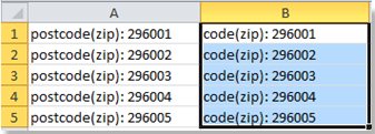
Step 2. Then press Enter key, and select the cell B1, then drag the fill handle over the cells that you want to contain this formula. And now you are successful in removing the first 4 characters of the text strings. See screenshot:



If you need to remove the last several characters, you can use the LEFT function as the same as the RIGHT function.

Note: Using the Excel function to remove certain characters is not as directly as it is. Just take a look at the way provided in next method, which is no more than two or three mouse clicks.

Remove First Or Last Characters By Find And Replace In Excel

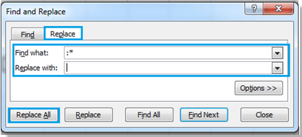
If you want to remove all characters at the front or end of the colon :, Find and Replace function in Excel also can make your removing as soon as quickly.

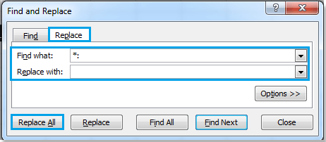
Step 1. Hold the Ctrl button and press F to open Find and Replace dialog, and click Replace.

Step 2. Enter :* into the Find what box, and leave blank in Replace with box. See screenshot:



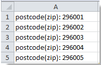
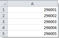
Step 3. Click Replace All, and all the characters at the end of the colon (include the colon) have been removed. See screenshot:



If you want to remove all characters before the colon, please type *: into the Find what box, and leave blank in Replace with box. See screenshot:



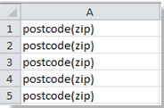
Click Replace All, all the characters before the colon have been removed. See screenshot:



Note: This method is only applied to the characters which contain the specific separators, so you can change the colon: to any other separators as your need.

https://www.extendoffice.com/documents/excel.html

Excel : How To Move Minus Sign From Right To Left/Back To Front In Excel?

Symptoms

When you import a worksheet into Microsoft Excel and that worksheet contains numbers with minus signs on the right (for example, 12345-), Microsoft Excel may not treat these numbers as negative numbers.

Cause

Microsoft Excel treats these numbers as text because the minus sign appears to the right side of the number.

Workaround

There are two ways to solve this problem:

1. Use a worksheet formula. -or-

2. Create a macro.

Use the following formula in a worksheet:

=IF(RIGHT(A1,1)="-","-"&LEFT(A1,LEN(A1)-1),A1)*1
=IF(RIGHT(A1,1)="-",SUBSTITUTE(A1,"-","")*-1,A1)
=VALUE(IF(RIGHT(A1,1)="-",RIGHT(A1,1)&LEFT(A1,LEN(A1)-1),A1))

For example, follow these steps:

1. Enter the following in a worksheet:

A1: 3

A2: 2-

A3: 1-

A4: 4

A5: 6-

2. In cell B1, enter the above formula.

3. Fill the formula in B1 down to B5.

4. Select cells B1:B5 and click Copy on the Edit menu.

5. Select cell A1 and click Paste Special on the Edit menu.

6. Click Values and click OK.

7. Select B1:B5 and click Delete on the Edit menu.

*******************************************************************************

There is a hidden utility in Text to Columns that can help you move minus sign from back to front.

1. Select the numbers you want to fix the trailing minus sign, and click Data à Text to Columns. 

2. In the Text to Columns wizard, directly click Next à Next to go to the Step 3 of 3 dialog, and click Advanced. 

3. In the Advanced Text Import Settings dialog, just check Trailing minus for negative numbers option, and click OK to close it.

4. Then click Finish to close Text to Columns dialog, and the minus sign of the negative numbers have been moved from back to front.

*******************************************************************************

If you are familiar with VBA, here is one can help you.

1. Press Alt + F11 keys simultaneously to open Microsoft Visual Basic for Applications window.

2. Click Insert à Module, and paste below VBA code to the new Module window.

VBA: Move minus sign from back to front (right to left)

Sub FixTrailingNumbers()

'UpdatebyKutoolsforExcel20160409

    Dim xRg As Range

    Dim xCol As Range

    Dim xTxt As String

    On Error Resume Next

    xTxt = ActiveWindow.RangeSelection.Address

    Set xRg = Application.InputBox("Select a range", "Kutools for Excel", xTxt, , , , , 8)

    If xRg Is Nothing Then Exit Sub

    For Each xCol In xRg.Columns

        xCol.TextToColumns Destination:=xCol, TrailingMinusNumbers:=True

    Next

End Sub

3. Click Run button or F5 key to execute this code, and a Kutools for Excel dialog pops out to remind you select a range to work. 

4. Click OK, and now the minus signs of negative numbers have been fixed correctly.

------------------***************------------------

https://www.extendoffice.com/documents/excel.html