Protect Macro

Command Button:-

Place a "Command Button" on your worksheet and add the following code lines:

1. On the Developer tab, click Insert.

2. In the ActiveX Controls group, click Command Button.



3. Drag a command button on your worksheet.

Assign a Macro:-

To assign a macro (one or more code lines) to the command button, execute the following steps.

1. Right click CommandButton1 (make sure Design Mode is selected).

2. Click View Code.



The Visual Basic Editor appears.

3. Place your cursor between Private Sub CommandButton1_Click() and End Sub.

4. Add the code line shown below.


Protect Macro

1. First, create a simple macro that you want to protect.

Range("A1").Value = "This is secret code"

2. Next, click Tools, VBAProject Properties...



3. On the Protection tab, check "Lock project for viewing" and enter a password twice.



4. Click OK.

5. Save, close and reopen the Excel file. Try to view the code.

The following dialog box will appear:



You can still execute the code by clicking on the command button but you cannot view or edit the code anymore (unless you know the password). The password for the downloadable Excel file is "easy".

6. If you want to password protect the macro from being executed, add the following code lines:

Dim password As Variant
password = Application.InputBox("Enter Password", "Password Protected")

Select Case password
    Case Is = False
        'do nothing
    Case Is = "easy"
        Range("A1").Value = "This is secret code"
    Case Else
        MsgBox "Incorrect Password"
End Select



Result when you click the command button on the sheet:

How to protect Excel sheet

To protect a sheet in Excel 2016, 2013 and 2010, perform the following steps.

1. Right click a worksheet tab at the bottom of your screen and select Protect Sheet… from the context menu.

Or, click the Protect Sheet button on the Review tab, in the Changes group.



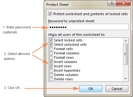
2. In the Protect Sheet dialog window, do the following:

To password protect your Excel sheet, type a password in the corresponding field. Be sure to remember the password or store it in a safe location because you will need it later to unprotect the sheet.

If the worksheet protection is nothing more than a precaution against accidental modification of the sheet contents by yourself or by the members of your local team, you may not want to bother about memorizing the password and leave the password field empty. In this case, unprotecting the sheet takes just a single click on the Unprotect Sheet button on the ribbon or in the sheet tab's right-click menu.

Select the actions you allow the users to perform.

• By default, the following 2 options are selected: Select locked cells and Select unlocked cells. If you leave only these two options selected, the users of your sheet, including yourself, will be able only to select cells (both locked and unlocked).
• To allow some other actions such as sorting, filtering, formatting cells, deleting or inserting rows and columns, check the corresponding boxes.
• If you don't check any action, users will only be able to view the contents of your Excel sheet.

Click the OK button.



3. The Confirm Password dialog box will pop-up prompting you to retype the password so that an accidental misprint won't lock your Excel sheet forever. Retype the password and click OK. Done!

How to unprotect Excel sheet with password

If you know the password for the protected sheet, removing protection is a matter of seconds. Just do any of the following:

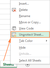
1. Right-click the sheet tab, and select Unprotect Sheet… from the context menu.



2. On the Review tab, in the Changes group, click Unprotect Sheet.



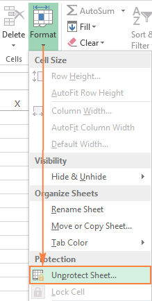
3. On the Home tab, in the Cells group, click Format, and select Unprotect Sheet from the drop-down menu.



If you are dealing with a password-protected worksheet, Excel will ask you to enter the password. Type the password and click OK.

If the worksheet was not protected with password, clicking the Unprotect Sheet button is all it takes to unlock the sheet.

How to unprotect Excel sheet without password

As mentioned in the beginning of this tutorial, Excel worksheet protection is quite weak even in the recent versions of Excel 2013 and Excel 2016. If you need to edit a password protected sheet but you cannot remember the password, try to unlock that Excel spreadsheet by using one of the following methods.

Unlock Excel spreadsheet with VBA code (for Excel 2010 and lower) :-

If you are using Excel 2010 or older version, you can unlock a password-protected sheet with the following macro.

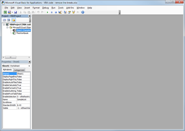
1. Press Alt + F11 to open the Visual Basic Editor.



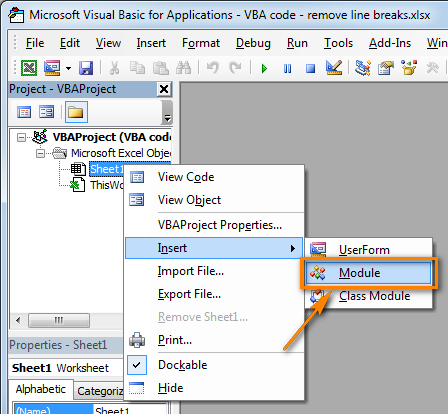
2. Right-click the workbook name on the left pane (Project-VBAProject pane) and select Insert > Module from the context menu.



3. Copy and paste the code below into the (Code) window. Do not change any of the code, just copy and paste it.

Sub PasswordBreaker()
    'Breaks worksheet password protection.
    Dim i As Integer, j As Integer, k As Integer
    Dim l As Integer, m As Integer, n As Integer
    Dim i1 As Integer, i2 As Integer, i3 As Integer
    Dim i4 As Integer, i5 As Integer, i6 As Integer
    On Error Resume Next
    For i = 65 To 66: For j = 65 To 66: For k = 65 To 66
    For l = 65 To 66: For m = 65 To 66: For i1 = 65 To 66
    For i2 = 65 To 66: For i3 = 65 To 66: For i4 = 65 To 66
    For i5 = 65 To 66: For i6 = 65 To 66: For n = 32 To 126
        ActiveSheet.Unprotect Chr(i) & Chr(j) & Chr(k) & _
            Chr(l) & Chr(m) & Chr(i1) & Chr(i2) & Chr(i3) & _
            Chr(i4) & Chr(i5) & Chr(i6) & Chr(n)
        If ActiveSheet.ProtectContents = False Then
            MsgBox "One usable password is " & Chr(i) & Chr(j) & _
                Chr(k) & Chr(l) & Chr(m) & Chr(i1) & Chr(i2) & _
                Chr(i3) & Chr(i4) & Chr(i5) & Chr(i6) & Chr(n)
            Exit Sub
        End If
    Next: Next: Next: Next: Next: Next
    Next: Next: Next: Next: Next: Next
End Sub

4. Press F5 or click the Run button on the toolbar and wait a couple of minutes. The macro will report a cracked password, which is not the original one (always some combination of A's and B's), but nevertheless it works. If you are not very comfortable with VBA, you can find the detailed guidance in the following tutorial: How to insert and run VBA code in Excel. If you need to unprotect Excel sheet without password in the modern versions of Excel 2013 and Excel 2016, try one of free tools, for example Password Protection Remover add-in for Excel.

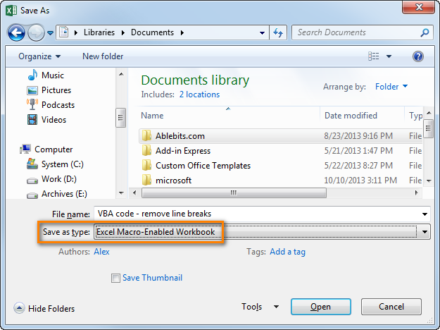
4. Save your workbook as "Excel macro-enabled workbook". Press Crl+S, then click the "No" button in the "The following features cannot be saved in macro-free workbook" warning dialog.

The "Save as" dialog will open. Choose "Excel macro-enabled workbook" from the "Save as type" drop-down list and click the Save button.

5. Press Alt+Q to close the Editor window and switch back to your workbook.

How to run VBA macros in Excel

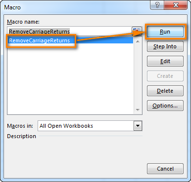
When you want to run the VBA code that you added as described in the section above: press Alt+F8 to open the "Macro" dialog.

Then select the wanted macro from the "Macro Name" list and click the "Run" button.

https://www.ablebits.com/office-addins-blog/2013/12/06/add-run-vba-macro-excel/

How to Protect Excel Workbook from Opening and Editing

Part 1:How to protect Excel workbook from opening

Add a Document Open Password for an Excel workbook so that all the users should type the correct password to open the workbook.

Step 1: In the opened Excel workbook, click on the File and select the Info. Click on the Protect Workbook button and select the Encrypt with Password from the expanded options.

Step 2: Type your password in the “Encrypt Document” dialog and click OK. Type the password again in the “Confirm Password” dialog and click OK to confirm.

Then the Excel Workbook has been protected from opening. A password will be required to open this workbook.

Part 2: How to protect Excel workbook from editing

You can mark an Excel workbook as Final or add password to protect the current sheet from being changed.

Way 1: Mark as Final

Step 1: Similarly click on the Protect Workbook button. Then select Mark as Final.

Step 2: Click on OK to confirm.

Now this Excel workbook has been marked as final to discourage editing. The users will be unable to edit in the cell. But there will be one yellow warning under the Excel tool bar. As long as the user clicks on the Edit Anyway, he can edit the Excel workbook. But the user had better not do this without the author’s permission if you are not the author.

Way 2: Protect current sheet

Step 1: Click on the Protect Workbook button and select Protect Current Sheet.

Step 2: In the Protect Sheet dialog, type the password to protect the worksheet. Under the Allow all users of this worksheet to, you can select the options to decide what types of changes the users can make to the worksheet.

Step 3: Type the password again to confirm.

Now the Excel workbook has been protected from editing. Once you attempt to modify the cell, it will prompt the warning message to tell the cell is protected and read-only. Only removing the password from the protected Excel workbook, can you modify the cell.

Another way to protect Excel workbook from opening and editing

Step 1: In an opened Excel workbook, click on File -> Save As.

Step 2: In the Save As dialog, click on the Tools button and select General Options.

Step 3: In the “General Options” dialog, you can set an Open password that protects the Excel workbook from opening and set a Modify password that protects the Excel workbook from editing.

How to show the Developer Tab in Excel

By default, the Developer Tab is not displayed as a menu option in Excel when you first open it up. You can, however, add it by following the few steps below.

Adding the Developer Tab to your Ribbon menu allows you to:

Write macros and VBA (Visual Basic for Applications) code.
Run macros that you previously recorded.
Use XML commands.
Use ActiveX controls.
Create applications to use with Microsoft Office programs.
Use form controls in Microsoft Excel.

Step 1 Click the File tab and then click Options



Step 2 Click Customize Ribbon.

Step 3 Under Customize the Ribbon and under Main Tabs, select the Developer check box and then click OK.



The Developer Tab will now show in the Ribbon Menu for you and will continue to show in Excel until you either reverse the instructions below or you reinstall Excel on your computer.

Excel : How to unprotect a password protected worksheet

In the case of a password protected worksheet where you are unable to Edit the data you can try the following steps to unprotect your worksheet.

Step 1: Press ALT +  F11 or click View Code on the Developers Tab

Step 2: Double click on the worksheet that is password protected.

Step 3: Copy and paste the code below into the (Code) window. Do not change any of the code, just copy and paste it.

Sub PasswordBreaker()
'Breaks worksheet password protection.
Dim i As Integer, j As Integer, k As Integer
Dim l As Integer, m As Integer, n As Integer
Dim i1 As Integer, i2 As Integer, i3 As Integer
Dim i4 As Integer, i5 As Integer, i6 As Integer
On Error Resume Next
For i = 65 To 66: For j = 65 To 66: For k = 65 To 66
For l = 65 To 66: For m = 65 To 66: For i1 = 65 To 66
For i2 = 65 To 66: For i3 = 65 To 66: For i4 = 65 To 66
For i5 = 65 To 66: For i6 = 65 To 66: For n = 32 To 126
ActiveSheet.Unprotect Chr(i) & Chr(j) & Chr(k) & _
Chr(l) & Chr(m) & Chr(i1) & Chr(i2) & Chr(i3) & _
Chr(i4) & Chr(i5) & Chr(i6) & Chr(n)
If ActiveSheet.ProtectContents = False Then
MsgBox "One usable password is " & Chr(i) & Chr(j) & _
Chr(k) & Chr(l) & Chr(m) & Chr(i1) & Chr(i2) & _
Chr(i3) & Chr(i4) & Chr(i5) & Chr(i6) & Chr(n)
Exit Sub
End If
Next: Next: Next: Next: Next: Next
Next: Next: Next: Next: Next: Next
End Sub

Step 4: Click on the Run Button or press F5.

Step 5: It will return you back to the worksheet and an alert box will appear with one usable password. Click OK and the Excel sheet will be unprotected immediately. You can modify the sheet without password.

What is the use of Trim formula?

Purpose              : Removes un-necessary spaces in a given text

Return value     : Text with extra spaces removed.

Syntax                 : =TRIM (text)

Parameter list   :  text - The text from which to remove extra space.

Example:

 Image 1a

 Image 1b

=TRIM(A1)  [Formula]

Cell A1 contains the string:

="James"&CHAR(32)&CHAR(32)&"Bond"&CHAR(160)&CHAR(160)&"007". 

Note that there are 2 spaces between " James" and "Bond" and then 2 spaces (nonbreaking space characters with decimal value of 160) between "Bond" and "007". The string Length - LEN(A1) - is 16 characters. Refer Image 1a.

Formula returns the string "James Bond  007". TRIM Function deletes one space between "James" and "Bond". Length of returned string is 15 characters. TRIM function does not remove the nonbreaking spaces represented by CHAR(160), which can be done by using the SUBSTITUTE function as shown below. Refer Image 1b.

=TRIM(SUBSTITUTE(A1,CHAR(160),CHAR(32)))  [Formula]

Replaces each nonbreaking space character (Unicode value of 160) with a space character (ASCII value of 32) by using the SUBSTITUTE function, and then removes the multiple embedded spaces from the above string in Cell A1 (Image 1a).

Formula returns the string "James Bond 007". Length of returned string is 14 characters. Refer Image 2.

LOOKUP Function

Syntax : LOOKUP(lookup_value,  lookup_vector,  [result_vector])

The LOOKUP function vector form syntax has the following arguments (argument: A value that provides information to an action, an event, a method, a property, a function, or a procedure.):

lookup_value Required. A value that LOOKUP searches for in the first vector. Lookup_value can be a number, text, a logical value, or a name or reference that refers to a value.

lookup_vector Required. A range that contains only one row or one column. The values in lookup_vector can be text, numbers, or logical values.

Important   The values in lookup_vector must be placed in ascending order: ..., -2, -1, 0, 1, 2, ..., A-Z, FALSE, TRUE; otherwise, LOOKUP might not return the correct value. Uppercase and lowercase text are equivalent.

result_vector Optional. A range that contains only one row or column. The result_vector argument must be the same size as lookup_vector.

What is the use of Length formula?

Purpose              :   Get the length of text.

Return value     :   A number representing the lengh of the text.

Syntax                 :   =LEN (text)

Parameter list   :   text - The text for which to calculate length.

Examples of Excel Len formula:

len("Shahul Hameed") = 13

len(A1) = length of the value in cell A1

To get the length of a string, use the LEN function.

Adding a Missing Closing Bracket

Use a formula to add any missing brackets. The following is just one example of the type of formula you can use:

=IF(AND(NOT(ISERROR(SEARCH("[",A1))),NOT(RIGHT(A1,1)="]")),A1&"]",A1)

The trick is to check to see if the cell (A1 in this case) has a left bracket in it and, if it does, check for the right bracket. If the right bracket isn't found, then you append one to the contents of the cell. Here's another variation on the same formulaic theme:

=IF(ISERROR(FIND("[",A1)),A1,IF(ISERROR(FIND("]",A1)),A1&"]",A1))

If you have to check large numbers of cells for missing brackets on a regular basis, you may want to create a macro that will examine a range of cells and add a right bracket if one is needed. Here's an example of how such a macro could be formulated:

Sub Close_Bracket()

    Dim c As Range

    Const csLBrk As String = "["

    Const csRBrk As String = "]"

    On Error Resume Next

    For Each c In Selection.Cells

        If InStr(1, c.Value, csLBrk) > 0 And _

          InStr(1, c.Value, csRBrk) = 0 Then

            c.Value = c.Value & csRBrk

        End If

    Next c

End Sub

To use the macro, simply select the range of cells you want to affect, and then run it. The cells are examined in-place and modified, if needed.